Since Gaussian integers are the coordinates of discrete square pixels in the complex plane, complex operations can be used to implement 2-D graphics operations. Many 2-D algorithms are more elegant in complex number form--e.g., one can envision a 2-D spreadsheet for scientific applications whose coordinates are Gaussian integers.
Many computer languages--e.g., Fortran-77, APL--incorporate complex numbers as a primitive datatype,[1] and some recent languages--e.g., Common Lisp, Scheme--incorporate rational numbers, as well. Unfortunately, these two datatypes have not been well integrated with each other in these computer languages, although mathematicians have known since the time of Gauss how such an integration may be accomplished by means of Gaussian integers--i.e., complex numbers whose real and imaginary parts are both ordinary (rational) integers.
Gaussian integers, in addition to their intrinsic mathematical interest, also serve as an important "test case" for theories of polymorphism in object-oriented programming, since Gaussian integers "inherit" from both the integers and the complex numbers, and since complex rational numbers can be seen either as Q[i] (the rationals extended with the complex number i, i^2=-1, i^4=1), or as the field of quotients of Gaussian integers (ratios of Gaussian integers analogous to the ratios of rational integers found in the field Q of the rational numbers).
We give code for the appropriate functions in Common Lisp, because it already has arbitrary-precision integers, arbitrary-precision rational numbers, and complex rational numbers, and therefore the incremental code required for incorporating Gaussian integers in Common Lisp is quite small relative to most other languages.
We suggest that facilities for Gaussian integers be included in generic complex number standards for arbitrary computer languages [Hodgson91]. Such facilities are in accord with the basic philosophy that if a primitive numeric datatype is provided at all, then all of the relevant primitive functions should be extended to deal with this datatype, so long as there is general agreement among mathematicians regarding the meaning of such extensions.
The Gaussian integers have a Euclidean greatest common divisor algorithm, and hence they form a Euclidean principle ideal domain.[2] They thus have a unique[3] factorization into Gaussian primes, which are the numbers: a) +-1+-i, b) ordinary (rational) integer primes of the form |p|=4k+3, and c) +-m+-ni, +-n+-mi, where m^2+n^2=4k+1=|p|, p an ordinary (rational) integer prime. Thus, in going from the ordinary (rational) integers to the Gaussian integers, each ordinary (rational) prime becomes either four (|p|=2, |p|=4k+3) or eight (|p|=4k+1) Gaussian primes, and these are the only Gaussian primes.
Plot of the Gaussian primes in the first quadrant.
We can now count the number of Gaussian integers which lie on a circle of radius sqrt(n) around the origin. If any prime of the form |p|=4k+3 appears with an odd exponent in the (rational) factorization of n, then the circle includes no Gaussian integers. Otherwise, let n=n0*n1*n3, where n0 contains all of the powers of 2, n1 contains all of the primes of the form |p|=4k+1, and n3 contains all of the primes of the form |p|=4k+3; the circle of radius sqrt(n) then contains 4*d(n1) points, where d(n1) is the number of (rational) divisors of n1. For example, there are no Gaussian integers on the circle of radius sqrt(7), but 4*(3+1)*(2+1)=48 Gaussian integers on the circle of radius sqrt(169000)=sqrt(2^3*5^3*13^2).
Since ordinary (rational) primes of the form |p|=4k+3 are also Gaussian primes, the ring of Gaussian integers Z[i] modulo p is isomorphic to the finite field Zp[x]/(x^2+1) of norm(p)=p^2 elements, since the polynomial x^2+1 is irreducible (non-factorable) over Zp [Lange70]. On the other hand, if |p|=4k+1, then the ring of Gaussian integers Z[i] modulo m+ni, where m^2+n^2=|p|, is a finite field of norm(m+ni)=|p| elements, which is therefore isomorphic to the finite field Zp [Lange70], but which folds up its structure in a more interesting 2-dimensional way.
(defun gaussian-integerp (z)
  (assert (numberp z))
  (and (integerp (realpart z)) (integerp (imagpart z))))
(defun norm (z)
  (realpart (* z (conjugate z)))) ; "realpart" needed only for non-Lisp langs.
When we divide complex numbers, however, we must now worry
about the phase of the divisor rather than just its
sign. We know that for a Gaussian integer divisor m+ni,
we need m^2+n^2 distinct remainders, so the most elegant choice of
representative remainders is a square of area m^2+n^2 which is
tilted at an angle of atan(n/m);[5]
equivalently, we consider the remainder fraction r/d to reside in an
upright square of area 1. The correct quotient for this
choice is computed by
q=divide(realpart(z*d^*),d*d^*)+i*divide(imagpart(z*d^*),d*d^*),[6] where "divide" is one of floor,
ceiling, truncate or round, and the correct
remainder is computed by r=z-q*d. This q produces the correct
remainder even when z,d are both real, so long as
divide(z,d)=divide(-z,-d). We give definitions for complex
floor and round; the other two are analogous. The
remainders r produced by the round function with a complex
divisor d do satisfy the requirement 0<=|r|<=|d|, but the
remainders from the other three functions do not satisfy this
requirement.
(defun complex-floor (z d)
  ;;; Should use defmethod on "floor", instead.
  (let* ((dc (conjugate d)) (dn (* d dc)) (zdc (* z dc)))
    (complex (floor (realpart zdc) dn) (floor (imagpart zdc) dn))))

(defun complex-round (z d)
  ;;; Should use defmethod on "round", instead.
  (let* ((dc (conjugate d)) (dn (* d dc)) (zdc (* z dc)))
    (complex (round (realpart zdc) dn) (round (imagpart zdc) dn))))
These functions do not exhaust the possibilities for Gaussian integer division.
Criteria for evaluating the possibilities are the following (see also
[McDonnell73] [Forkes81]):
floor remainders (mod 3+2i) (black) and (mod (3+2i)*(3-2i)=13) (grey); i = 5 (mod 3+2i).
(defun gaussian-gcd1 (z1 z2)
  ;;; Compute gcd using Euclidean algorithm and least abs remainders.
  (let* ((nz1 (norm z1)) (nz2 (norm z2)))
    (if (< nz1 nz2) (gaussian-gcd1 z2 z1)
      (if (= nz2 0) z1
        (gaussian-gcd1 z2 (- z1 (* z2 (complex-round z1 z2))))))))

(defun gaussian-gcd (z1 z2)
  ;;; Should use defmethod on "gcd", instead.
  ;;; Fix up result of gaussian-gcd1 using units.
  (let* ((g (gaussian-gcd1 z1 z2))
         (gr (realpart g)) (gi (imagpart g)))
    (cond ((plusp gr) (if (minusp gi) (* (complex 0 1) g) g))
          ((minusp gr) (if (plusp gi) (* (complex 0 -1) g) (- g)))
          (t (abs gi)))))

(defun gaussian-lcm (z1 z2)
  ;;; Should use defmethod on "lcm", instead.
  (/ (* z1 z2) (gaussian-gcd z1 z2)))
The convergence of this gcd algorithm requires that the complex round
function fit a square peg--the set of remainders
{x+yi=z-d*round(z,d)}--into a round hole
{x^2+y^2<norm(d)}. Slowly converging Gaussian gcd's can be
constructed from a Gaussian Fibonacci sequence: i, 1+i,
1+2i, 2+3i, 3+5i, ..., F[k]+iF[k+1], where
F[k] is the k'th Fibonacci number [Harmon81]. Gaussian Fibonacci
numbers have a Fibonacci norm:
norm(F[k]+iF[k+1])=F[k]^2+F[k+1]^2=F[2k+1]. Furthermore,
F[2k]^2=F[2k-1]^2=-1 (mod F[2k+1]), so we have an explicit formula for
i: i=F[2k] (mod F[2k+1]).
Divisibility of a number z by 1+i is equivalent to divisibility of
norm(z) by 2, so we can more efficiently check for the evenness of norm(z).
But we can do even better [Knuth81,4.1#28ans]. If z=m+ni, then
norm(m+ni) is even if and only if m^2 and n^2 are both odd or both even.
But m^2 is even if and only if m is even so norm(m+ni) is even if and
only if m and n are both odd or both even. Furthermore, m+n is even if and
only if m and n are both odd or both even. Finally, z=m+ni is even if
and only if m+n is even.
(defun gaussian-evenp (z)
  ;;; Should use defmethod on "evenp", instead.
  (evenp (+ (realpart z) (imagpart z))))

(defun gaussian-oddp (z)
  ;;; Should use defmethod on "oddp", instead.
  (not (gaussian-evenp z)))
The numerator and denominator functions can be extended to any complex number whose real and imaginary parts are rational numbers by using the gaussian-gcd algorithm given above to reduce the numerator and denominator to lowest terms. We must also canonicalize the denominator to the region of the positive real axis and the first quadrant by multiplying by i, except when the gcd is real. We note that gaussian-numerator and gaussian-denominator are not trivial functions--e.g.,
(gaussian-numerator (complex 3/25 -4/25)) = 1 and
(gaussian-denominator (complex 3/25 -4/25)) = (complex 3 4).
(defun gaussian-numerator (z)
  ;;; Should used defmethod on "numerator", instead.
  (let* ((x (realpart z)) (y (imagpart z))
         (xd (denominator x)) (yd (denominator y))
         (zn (complex (* (numerator x) yd) (* (numerator y) xd)))
         (zd (* xd yd)) (g (gaussian-gcd zn zd)) (r (/ zn g)))
    (if (zerop (imagpart g)) r (* (complex 0 1) r))))

(defun gaussian-denominator (z)
  ;;; Should use defmethod on "denominator", instead.
  (let* ((x (realpart z)) (y (imagpart z))
         (xd (denominator x)) (yd (denominator y))
         (zn (complex (* (numerator x) yd) (* (numerator y) xd)))
         (zd (* xd yd)) (g (gaussian-gcd zn zd)) (r (/ zd g)))
    (if (zerop (imagpart g)) r (* (complex 0 1) r))))
Wilson's Theorem tells us that (p-1)! = -1 (mod p),[14] and if p=4k+1 then ((2k)!)^2 = -1 (mod p),[15] so we have an explicit solution h = mod((2k)!,p)[16] to the equation h^2 = -1 (mod p). Since h^2+1=(h+i)*(h-i)=t*p, for some integer t<p, there must be a non-trivial factor m+ni in common between h+i and p, and yet this factor cannot be p itself, because t*p<p^2. Therefore, gcd(h+i,p)=m+ni is one of the prime factors of p that we seek [Knuth81,3.3.4#11].[17] The other factor is m-ni, and any other factorization of p is produced by including unit factors of the forms +-1 and +-i.
For example, take the prime 53=4*13+1. Now 23^2 = -1 (mod 53), or equivalently, 23^2+1 = 10*53, so t=10=2*5 (any odd prime factor q of t with exponent 1 must also be of the form 4k+1, otherwise we have produced a square root of -1 (mod q), which is impossible for primes not of the form 4k+1). Computing the gcd of 23+i and 53, we get 2+7i, so m= +-2, n= +-7 for p=53.
Most graphics texts--e.g., [Newman79]--treat the 2-D pixel plane in terms of real vectors rather than complex numbers. While this vector algebra approach--first popularized by Gibbs--extends easily to 3 (and higher) dimensions, it ignores the profoundly different characters of 2-D and 3-D spaces. For example, polynomial equations of even degree with real coefficients may not have any real roots, while such equations of odd degree always have at least one real root; this simple difference means that nontrivial rotations of a "sphere" in 2-D have no fixed points at all, while nontrivial rotations of a sphere in 3-D always have a fixed pole. Physicists and electrical engineers know that the wave equation preserves impulses (Huyghen's principle) only for odd-dimensional spaces--e.g., the wave equation in 2-D has an infinite impulse response, whereas in 3-D it obeys Huyghen's principle [Courant62]. Therefore, when working in 2-D, one should take advantage of the special characteristics of 2-D and utilize the most powerful representation possible--i.e., the complex number--without worrying about whether it extends to higher dimensions.[18] For example, the additional algebraic structure of the complex multiplicative inverse gives us the Möbius transforms (A*z+B)/(C*z+d), where A,B,C,D are complex constants, which provide us with elegant uniform representations for lines and circles in the complex plane [Schwerdtfeger62]. This algebraic structure also gives us a complex "interval arithmetic" in which the "intervals" are small circular disks [Gargantini72].
An interesting coordinate transformation for such a 2-D image is the log-polar transform, which takes the pixel at x+yi and maps it to the position log(x+yi) = log|x^2+y^2|+i atan(y/x). After such a "texture-mapping" operation, the image can be size- and rotation-normalized by simple translation operations, making image recognition easier.
Another elegant way to represent a closed contour on the complex plane (whether it interseects itself or not) is by means of Fourier descriptors [Pavlidis77]. If the contour is approximated by means of a list of points x+yi which are (approximately) equally spaced in terms of path length, then a one-dimensional Fourier transform of that list provides an equivalent representation, which can be less sensitive to rotation and scaling. Contour shapes can be approximated by keeping only the coefficients for the lower frequencies--e.g., 15 harmonics are sufficient to preserve recognizable shapes for the digits 0-5 [Brill68]. For simple shapes in which the entire boundary is "visible" from the origin--i.e., the boundary is a single-valued function in polar coordinates--the boundary points for the Fourier transform can be chosen at equal angles around the origin.
As an example of a very simple shape, a circle can be represented by the parameterization C0+R*exp(i*2*pi*t), where C0 is the center of the circle, and R is a real number radius--i.e., circles can be represented by only 2 harmonics.
Consider, for example, the Gaussian prime 10+i whose norm is 101. In
order to demonstrate a raster scan, we will define the modulo function
to be used for computing (mod 10+i) as follows:
(defun modulo (z d)
  ;;; Modulo function for doing raster scans.
  ;;; This modulo function won't work for computing gcd's.
  (- z (* d (complex-floor z d))))
The above modulo function does not produce a result whose norm
is smaller than the divisor, but it does "tile the plane". Each of these
tiles, when considered as a pattern of discrete pixels, forms an L-shaped tile
consisting of a 10x10 square above a 1x1 square, as might be expected from the
fact that 101=10^2+1^2. This familiar tiling pattern repeats on an angle of
atan(1/10).[22]
If we now compute 0 (mod 10+i), 1 (mod 10+i), 2 (mod 10+i), 3 (mod 10+i), ..., 100 (mod 10+i), then we get the following "inverse table", where the number at position x+yi indicates the integer 0-100 that maps to x+yi.
10i |  1    2    3    4    5    6    7    8    9   10
 9i | 11   12   13   14   15   16   17   18   19   20
 8i | 21   22   23   24   25   26   27   28   29   30
 7i | 31   32   33   34   35   36   37   38   39   40
 6i | 41   42   43   44   45   46   47   48   49   50
 5i | 51   52   53   54   55   56   57   58   59   60
 4i | 61   62   63   64   65   66   67   68   69   70
 3i | 71   72   73   74   75   76   77   78   79   80
 2i | 81   82   83   84   85   86   87   88   89   90
 1i | 91   92   93   94   95   96   97   98   99  100
 0i |  0
    -------------------------------------------------
       0    1    2    3    4    5    6    7    8    9
Table of n (mod 10+i), for n = 0 (1) 100, showing raster scan pattern.
If we start counting with 1, then our raster scan will start at the top left corner (0+10i) and sweep out successive rows of pixels on our Gaussian screen whose upper left hand corner is 0+10i and whose lower right hand corner is 9+i. The number 101 maps to the same pixel as the number 0--i.e., the pixel 0+0i, which acts as a kind of "vertical retrace" pixel. Even more interestingly, we can do a vertical raster scan by using the series 0i, 1i, 2i, 3i, ..., etc. (mod 10+i)--i.e., the series Zi. In fact, we can produce almost any conceivable scan of this "square" by considering the series Z*k, for any Gaussian integer k, and scans without a "retrace pixel" can be made by considering the powers of primitive elements (see [Brenner73] and [Baker74] ).
Gaussian primes of the form m+i appear to be moderately common--e.g., there are about 50 whose norms are less than 100,000. Particularly interesting are the Gaussian factors of Fermat primes of the form 2^(2^n)+1. For example, the Fermat prime 65,537 splits into Gaussian factors 256+-i, which gives us a 256x256 Gaussian graphics screen. Unfortunately, there may be only 5 Fermat primes, of which 65,537 is the largest known, and it is conjectured that these 5 are all that exist [Hardy79]. It is not known if there are more than a finite number of primes of the form m^2+1 [Hardy79], although--unlike Fermat primes--these primes are empirically rather easy to find.
For example, each of the following integers m produces a prime p=m^2+1.
2, 4, 6, 10, 14, 16, 20, 24, 26, 36, 40, 54, 56, 66, 74, 84, 90, 94, 110, 116, 120, 124, 126, 130, 134, 146, 150, 156, 160, 170, 176, 180, 184, 204, 206, 210, 224, 230, 236, 240, 250, 256, 260, 264, 270, 280, 284, 300, 306, 314, 326, 340, 350, 384, 386, 396, 400, 406, 420, 430, 436, 440, 444, 464, 466, 470, 474, 490, 496, 536, 544, 556, 570, 576, 584, 594, 634, 636, 644, 646, 654, 674, 680, 686, 690, 696, 700, 704, 714, 716, 740, 750, 760, 764, 780, 784, 816, 826, 860, 864, 890, 906, 910, 920, 930, 936, 946, 950, 960, 966, 986, 1004, 1010, 1036, 1054, 1060, 1066, 1070, 1080, 1094, 1096.
[ a b e ]   [x]   [ a*x+b*y+e ]
[ c d f ] * [y] = [ c*x+d*y+f ]
[ 0 0 1 ]   [1]   [     1     ]
Affine transformations in the complex plane can also be accomplished by means
of complex arithmetic:
affine(z) = A*z + B*z^* + C, where A, B, C are complex constants and z^* = conjugate(z).
This general form is preserved when composing affine transformations, as can be readily checked with simple algebra. That this general form can accomplish any affine transformation can be seen by converting the homogeneous matrix form of affine transformation into the complex form. If a,b,c,d,e,f are the parameters of the transformation matrix, as above, then we can express the complex constants A,B,C in terms of a,b,c,d,e,f:
A = ((a+d)-(b-c)i)/2, B=((a-d)+(b+c)i)/2, C=e+fi
Unlike the case with homogeneous matrices, the complex form of an affine transformation is particularly perspicuous when it comes to rotations. If we have a transformation which is just a proper rotation (i.e., without a flip), then A=exp(i*theta), where theta is the angle of rotation, and B=C=0. If we have an improper transformation which involves a flip, then B=exp(i*theta), where theta is the angle of rotation, and A=C=0. Thus, for proper Euclidean transformations, |A|=1 and B=0.
theta = sum(k=0,infinity,d[k]*a[k]) = sum(k=0,infinity,d[k]*atan(2^(-k))).
Equivalently, we can express a rotation exp(i*theta) as an infinite product of complex factors--i.e.,
exp(i*theta) =
sum(k=0,infinity,((2^k+i)^d[k])/abs((2^k+i)^d[k])) =
sum(k=0,infinity,(2^k+d[k]*i)/sqrt(2^(2k)+1))) =
1/K * sum(k=0,infinity,(1+d[k]*2^(-k)*i)),
where the factor K = sqrt(product(k=0,infinity,(1+2^(-2k)))) ~ 1.64676
is a normalization constant[23] independent of theta. Therefore, any rotation can be factored into a series of additions and shifts (followed by a single normalization) in a manner reminiscent of the decomposition of normal multiplication into additions and shifts. The binary digits d[k] = +-1 are found by a binary search of a virtual table of arctangents of powers of 2. Only 1 bit needs to be stored for each factor in the product, thus providing a compact code for rotations.
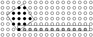
It should be no surprise, then, that the design of raster graphics 2-D frame buffers can benefit from the properties of the Gaussian integers. Modern 2-D frame buffers must be designed in such a way that groups of adjacent pixels in a single scan line can be accessed from the frame buffer in a single memory cycle to refresh the display, which implies that each pixel in the group must be stored in a separate memory chip. However, most graphics algorithms access the frame buffer in patterns which have locality in two dimensions, which implies that each pixel in a small 2-D neighborhood should be stored in a separate memory chip. Both of these properties are elegantly satisfied by using a Gaussian modulo function for the mapping of 2-D coordinates to memory chips--e.g., chip#(x,y) = mod(x+yi,m+ni), where m,n are rational integer constants, and gcd(m,n)=1. For example, if m+ni=3+2i, then 3^2+2^2=13 memory chips are required, and the two access patterns are shown in the figure of section E, above Furthermore, access to any square of the fundamental size and orientation--regardless of its translation--can be performed in a single memory cycle, and these pixels can then be permuted to standard positions using a cyclic barrel shifter. In the above example, consider accessing the tilted square whose bottom corner is located at 1+2i. Then the fundamental slice is cyclically shifted left by 1+2i=1+2*5=11, since i=5 (mod 3+2i).
Gaussian integer constants of the form 2^k+i are particularly appropriate for such memory systems. These moduli involve computing mod(x,2^(2k)+1), which can be done by the binary equivalent of "casting out elevens"--i.e., trivially express x in base-2^(2k) notation, and then alternately add and subtract each big digit. This procedure works because (2^(2k))^j = (-1)^j = +-1 (mod 2^(2k)+1).
[Chor86] effectively suggests the use of Fibonacci Gaussian integer constants F[k]+iF[k+1] for raster graphics memory systems, because Fibonacci systems provide interference-free access to rectangles of the largest area.
Memory cache designs can be optimized for 2-D access by means of these mapping techniques. Even with no special hardware, software mappings of this kind can optimize existing caches. Cache "lines" then become cache "squares"!
We prefer the use of tilted squares for representing the remainders of complex division, rather than the rectangles of APL. Square residue sets seem to offer the most elegant utilization of the two real parameters (real and imaginary parts) implicit in a complex divisor--as defining the size and orientation of the square. Different division functions are useful in different contexts, however, so we recommend that a multiplicity of division functions be provided.[28]
If one prefers hexagonal pixels to square pixels, this paper can be rewritten to uniformly utilize the ring Z[w]=Z+Z*w instead of the Gaussian ring Z[i], where w is a primitive root of unity--i.e., w^6=1 (where w = (1+-sqrt(3)i)/2) instead of i^4=1. The Euclidean gcd algorithm works in this ring with norm(m+nw)=m^2+m*n+n^2. The basic lattice is equilateral triangular, and the remainders can be made to tile the plane with hexagons [Hardy79]. Such a tiling is ideal for the RGB triads of a color television, because the lattice points (pixels) then fall into exactly three classes-- = 0, +1, -1 (mod (2w-1)=sqrt(3)i).
[Baker74] Baker, H.G. "On the Permutations of a Vector Obtainable through the Restructure and Transpose Operators of APL". 1974, published recently in APL Quote Quad 23,2 (Dec. 1992), 27-31.
[Baker92] Baker, H.G. "Computing A*B (mod N) Efficiently in ANSI C". Sigplan Not. 27,1 (Jan. 1992), 95-98.
Beeler, M., et al. "HAKMEM". MIT AI Memo 239, Feb. 29, 1972. See items #107,136-138.
Bracewell, R.N. The Fourier Transform and Its Applications, 2nd. Ed. McGraw-Hill, NY 1986.
Brenner, N. "Algorithm 467: Matrix transpose in place". CACM 16,11 (1973), 692-694.
Brill, E.L. "Character Recognition via Fourier Descriptors". Proc. WESCON Paper 25/3, Los Angeles, 1968.
Chor, B., et al. "An Application of Number Theory to the Organization of Raster-Graphics Memory". JACM 33,1 (Jan. 1986), 86-104.
Courant, R., and Hilbert, D. Methods of Mathematical Physics, Vol. II. Wiley & Sons, New York, 1962.
Davenport, H. The Higher Arithmetic: An Introduction to the Theory of Numbers, 6th Ed. Camb. U. Press, 1992.
Diaz, B.M., and Bell, S.B.M., eds. Spatial Data Processing using Tesseral Methods. Nat. Envir. Res. Council, Swindon, 1986.
Duprat, J., et al. "New Redundant Representations of Complex Numbers and Vectors". IEEE Trans. Computers 42,7 (July 1993), 817-824.
Eggleton, R.B., et al. "Euclidean Quadratic Fields". AMM 99,9 (Nov. 1992), 829-837.
Forkes, D. "Complex Floor Revisited". APL'81, ACM APL Quote Quad 12,1 (Sept. 1981), 107-111.
Gargantini, I., & Henrici, P. "Circular Arithmetic and the Determination of Polynomial Zeros". Numer. Math 18 (1972), 305-320.
Goffinet, D. "Number Systems with a Complex Base: a Fractal Tool for Teaching Topology". AMM 98,3 (Mar. 1991), 249-255.
Grünbaum, B., and Shepard, G.C. Tilings and Patterns. W.H.Freeman & Co., New York, 1987.
Hardy, G.H., and Wright, E.M. An Introduction to the Theory of Numbers, 5th Ed. Clarendon Press, Oxford, 1979.
Harmon, C.J. "Complex Fibonacci Numbers". Fibonacci Quart. 19,1 (Feb. 1981), 82-86.
Hodgson, G.S. "Rationale for the Proposed Standard for Packages of Real and Complex Type Declarations and Basic Operations for Ada". ACM Ada Letters XI, 7 (Fall 1991), 131-139.
Holladay, T.M. "An Optimum Algorithm for Halftone Generation for Displays and Hard Copies". Proc. Soc. Info. Disp. 21,2 (1980), 185-192.
Hurwitz, A. "Uber die Entwicklung Complexer Grossen in Kettenbruche". Acta Math. 11 (1888).
Knuth, D.E. The Art of Computer Programming, Vol. 2: Seminumerical Algorithms, 2nd Ed. Addison-Wesley 1981.
Kota, K., and Cavallaro, J.R. "Numerical Accuracy and Hardware Tradeoffs for CORDIC Arithmetic for Special-Purpose Processors". IEEE Trans. Computers 42,7 (July 1993), 769-779.
Kuck, D.J. The Structure of Computers and Computations, Vol. I. John Wiley & Sons, New York, 1978.
Lang, Serge. Algebra. Addison-Wesley, Reading, MA 1970.
McDonnell, E.E. "Complex Floor". Proc. APL Congress 73, North-Holland, Amsterdam, 1973.
McIlroy, M.D. "Best Approximate Circles on Integer Grids". ACM Trans. Graphics 2,4 (Oct. 1983), 237-263.
Middleditch, A.E. "Intersection Algorithms for Lines and Circles". ACM Trans. Graphics 8,1 (Jan. 1989), 25-40.
Newman, W.M., and Sproull, R.F. Principles of Interactive Computer Graphics. McGraw-Hill, New York, 1979.
Ore, Oystein. Number Theory and its History. McGraw-Hill, New York, 1948.
Pavlidis, T. Structural Pattern Recognition. Springer-Verlag, Berlin 1977.
Pavlidis, Theo. Algorithms for Graphics and Image Processing. Computer Science Press, Rockville, MD, 1982.
Pavlidis, T. "Curve Fitting with Conic Splines". ACM Trans. Graphics 2,1 (Jan. 1983), 1-31.
Penfield, P. "Principle Values and Branch Cuts in APL". Proc. APL81, APL Quote Quad 12,1 (Sept. 1981).
Penney, W. "A 'Binary' System for Complex Numbers". JACM 12,2 (Apr. 1965), 247-248.
Rokne, J.G., et al. "Fast Line Scan-Conversion". ACM Trans. Graphics 9,4 (Oct. 1990), 376-388.
Samet, H. "Hierarchical Representations of Collections of Small Rectangles". ACM Comput. Surv. 20,4 (Dec. 1988),271-309.
Schwerdtfeger, Hans. Geometry of Complex Numbers: Circle Geometry, Moebius Transformation, Non-Euclidean Geometry. Dover Publs., New York, 1962.
Shallit, J.O. Integer Functions and Continued Fractions. Princeton Univ., 1979.
[Steele90] Steele, Guy L. Common Lisp, the Language, 2nd Ed. Digital Press, Bedford, MA, 1990, 1029p.
Stein, S.K. "Algebraic Tiling". Amer. Math. Monthly 81 (1974), 445-462.
Turkowski, K. "Anti-Aliasing through the Use of Coordinate Transformations". ACM Trans Graph 1,3 (1982), 215.
Volder, J.E. "The CORDIC Trigonometric Computing Technique". IRE Trans. Elect. Comps. EC-8 (Sept. 1959).
Wagon, S. "The Euclidean Algorithm Strikes Again". AMM 97,2 (Feb. 1990), 125-129.
Wall, H.S. Analytic Theory of Continued Fractions. Chelsea Publ. Co., NY, 1948, 1973.
[1] As attractive as they are, Mandelbrot pictures are not the only use for complex numbers--e.g., trigonometry without complex numbers gives me a severe case of sinusitis (sinus is German for sine).
[2] An ideal is a subset I of a ring R which is closed under subtraction (I-I=I) and multiplication by arbitrary elements of the parent ring (R*I=I). In a principal ideal domain D, every ideal I can be represented as the set of multiples of a single generator element g--i.e., I=D*g. Every ideal of Z[i] is a magnified and tilted version of the square lattice Z[i].
[3] Clearly, any number of units can be introduced into a factorization.
[4] We strongly recommend against extending the relational operations--e.g., <,>,<=,>=--to the complex numbers by means of comparing absolute values or norms, as has been proposed by some in the Lisp and C++ communities. This is because these relational operators would then become discontinuous functions across the negative real axis.
[5] This choice of representatives is different from that in [McDonnell73] and [Forkes81], for reasons given below. The edges of these squares would make Bresenham [Newman79] proud.
[6] The multiplication of both the dividend and the divisor by a normalization factor (in this case d^*) is reminiscent of Knuth's Algorithm D [Knuth81,4.3.1].
[7] The set of remainders of a complex division by a divisor d need not be convex or even connected--e.g., any set S of complex numbers which represents every domain point (D=d*D+S), will work as a set of remainders [Goffinet90].
[8] Each (mod d) tile has area norm(d). However, the individual tiles may have non-convex fractal shapes such as the "twindragon" curves produced by bit strings interpreted as numbers of base i-1 [Knuth81,4.1]. Note that Common Lisp's round and truncate do not produce unique remainders, and therefore do not tile the plane. To tile the plane with hexagons instead of squares, utilize the ring Z[w]=Z+Z*w instead of Z[i], where w^3=-1 [Hardy79]. Square tiles can include only 2 edges and 1 corner; hexagonal tiles can include only 3 edges and 2 corners [Grünbaum87].
[9] Voronoi regions around the lattice points give the tiles with the least remainders; in Z[i], these regions are squares.
[10] [McDonnell73]'s complex floor function fails this criterion because its remainders form rectangles, not squares.
[11] ceiling can be used to encode base i-1 numbers whose digits are the bits 0,1. However, quater-imaginary numbers (base 2i) can't be handled by the usual APL-style encode function, since it produces imaginary digits--e.g., 1+i. Quadtrees [Samet88] are equivalent to base-2 numbers with the digits 0, 1, i, 1+i, which are gotten by interlacing the binary digits of the real and imaginary parts of a Gaussian integer.
[12] [Hurwitz88] suggests a complex round-like function based on the real function divide(x,d)=floor(x+d/2,d), which minimizes the size of remainders, but--unlike Common Lisp's round--produces unique representative remainders.
[13] Adding +-1+-i preserves parity, proving that chess bishops retain parity. Similarly, the fact that 2+i and 2-i are distinct primes, and hence gcd(2+i,2-i)=1, proves that chess knights can get to every square on an infinite chessboard.
[14] Proof: take the numbers 1,2,...,p-1 in pairs x,y, x/=y, such that x*y=1 (mod p). The only numbers left over will be 1 and -1, so the entire product will be = -1 (mod p).
[15] Proof: take the numbers 1,2,...,p-1 in pairs x, p-x, such that x*(p-x) = -x^2 (mod p). Since p=4k+1, there are an even number (2k) of such pairs, so we can rearrange the product of all of them as ((2k)!)^2. But this is the same product as in Wilson's theorem, which we have already shown to be = -1 (mod p).
Since squaring (mod p) is easier than computing factorials (mod p), we can more quickly find a quadratic non-residue c, such that c^(2k)=(c^k)^2=-1 (mod p), and thus h=c^k (mod p) [Wagon90].
[16] Don't compute the factorial before reducing mod p; do reduce mod p for every product [Baker92]; do use x-p if x>=p/2.
[17] Gauss gave explicit formulae for m,n: m = ((2k)!)/(2(k!)^2) (mod p) and n = (2k)!*m (mod p), where the m,n have the smallest absolute values [Davenport92]. This method for finding m,n is not at all obvious or as easy to remember as the gcd method.
Legendre used the continued fraction expansion (with a possibly long cycle) of sqrt(p) to produce m,n [Davenport92].
[Wagon90] shows that the gcd algorithm applied to the rational integers p,h produce m,n as the first two remainders less than sqrt(p). His method produces exactly the same intermediate results as the Gaussian gcd method, however.
[18] Hamilton's quaternions are elegant extensions of the complex numbers useful in 3-D and 4-D, but multiplication isn't commutative [Altmann86]. Quaternions are most conveniently manipulated as pairs of complex numbers.
[19] Gaussian graphical algorithms work best with square pixels, but then so do most graphics algorithms.
[20] If another division function is used, the shape of this array of pixels may be changed.
[21] That this scan of the square "fills the space" of pixels should not be surprising. König's corollary to Kronecker's Theorem [Hardy79] tells us that a reflected ray which makes an angle--whose tangent is irrational--to the side of a square with reflecting sides will densely and uniformly explore the interior of the square. In the present case of a rational tangent n/m, and a square of area m^2+n^2, an initially horizontal ray will be uniformly periodic with only integer-valued horizontal lines. There will also be a ruling of non-horizontal lines at angle 2*atan(n/m), which we conjecture will never intersect the lattice points inside the square. Thus, our fundamental square can be considered to be a "folded-up" version of the horizontal linear strip of height 1 and length m^2+n^2.
[22] Rational primes like p=m^2+n^2=norm(m+ni), m>n>1, give rise to tilings with a greater tilt.
[23] The product inside the radical is a generating function evaluated at 1/4 for distinct partitions of integers [Hardy79]. W. Gosper can accelerate convergence but is not aware of any simple "closed-form" representation for this constant.
[24] We will not discuss a mechanism for choosing the particular pixels to be turned on in each group.
[25] Gaussian bells that ring accidentally!
[26] These ideas are from [Holladay80] and [Chor86], which could both benefit handsomely from Gaussian integers.
[27] We assume that pitches and angles can be tightly controlled during fabrication, but not necessarily registration. However, registration in a Pythagorean chip should not matter very much!
[28] To paraphrase Emerson, "foolish consistency is the hobgoblin of little languages".